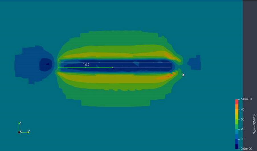
1.Resample with dataset
In this step we will discuss a few different ways to get data from the model.
To begin it is assumed that the following steps have been completed:
a. Stope Geometry has been loaded into ParaView.
b. CSV data loaded into Paraview. In this case, differential stress data has been used.
c. the Table to Points filter has been run on the imported csv data.
d. the Point Volume Interpolator has been run on the Table to Points filter.
e. An appropriate colour map has been applied. In this case the Preset used is erdc_rainbow_dark and the scale has been adjusted to values between 0 and 50 MPa. The opacity between 0 and 20MPa has been set to 0 for clearer viewing of the volume.
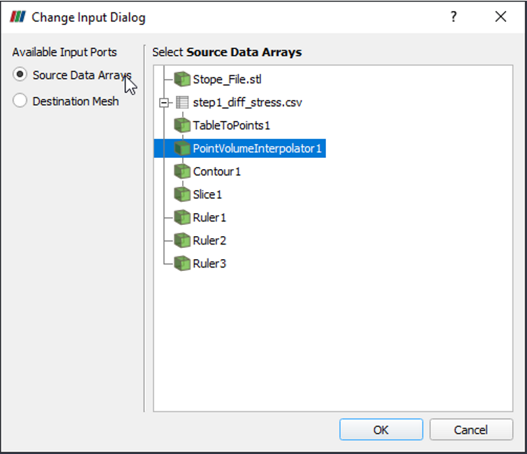
Start with the Point Volume Interpolator filter and then, right click to add a new filter. The filter that we want to add is called the resample with dataset filter. This filter will paint the result of the volume interpolator onto the original stope geometry.
Select the interpolator as the source array.
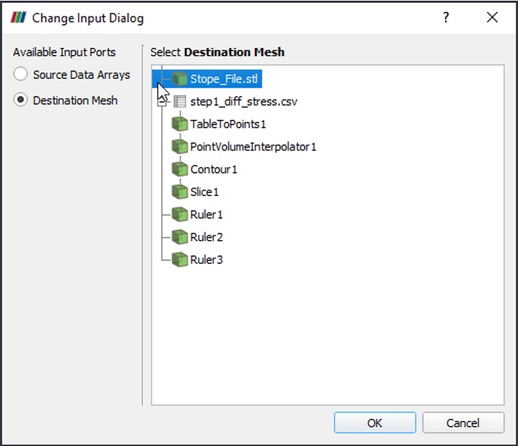
Then select the Stope_File as the Destination mesh.
The result is shown below.
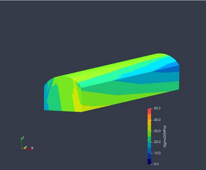
Note that the discretization in the Color Map Editor is turned on in this case. Turning it off will cause the image to have a smoother colour scheme.
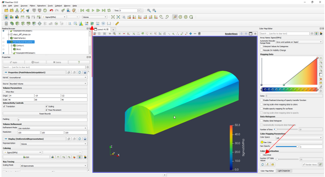
Turn off the discretization if you wish, but you may wish to leave it off in this case for a better looking image.
2. Using Plot over line
We may wish to visualise the strain over the length of the stope wall as a line graph. To do this, we need to use the Plot over Line tool which can be found in the top menu bar.
Recall that just like the Ruler, the ends of the line can be set by pushing ctrl+1 and ctrl+2 causing them to snap to the geometry. You can use this method to snap the measurement line to the geometry and then adjust the points manually. In this case the Z position of both points has been adjusted to 1.5mm.
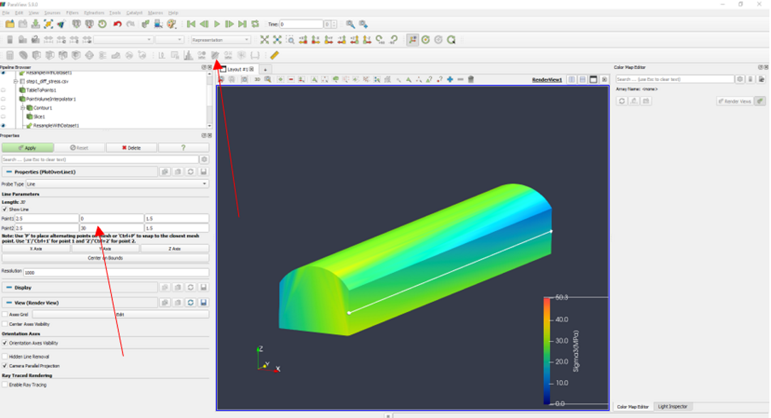
Clicking Apply here will create another window. In this window you will see a line graph representing the values encountered by the line as it moves across the stope. Note that you can change the axis of this line graph on the condition that you have the Plotoverline filter selected and that you scroll down in the properties window.
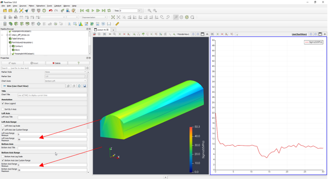
There is an interesting point on this graph at the position, 14.28m.
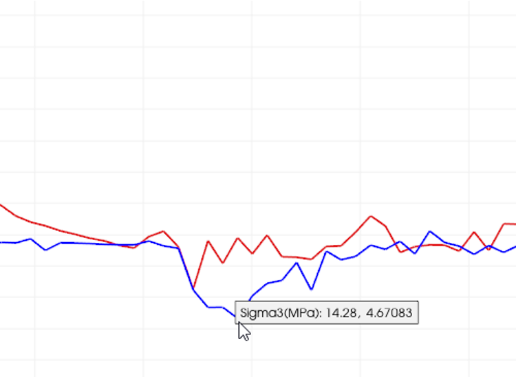
To get a look at a specific point on the model, you can use the probe tool.
To probe this location, first select the PlotOverLine1 filter in the pipeline browser. Then select the probe location tool.
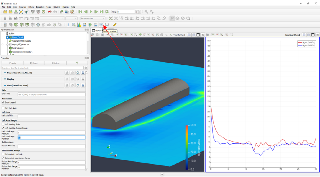
We can then set the position of the point, by pushing ctrl+P closest to where the datapoint is, then manually updating the sphere parameters to the exact location.
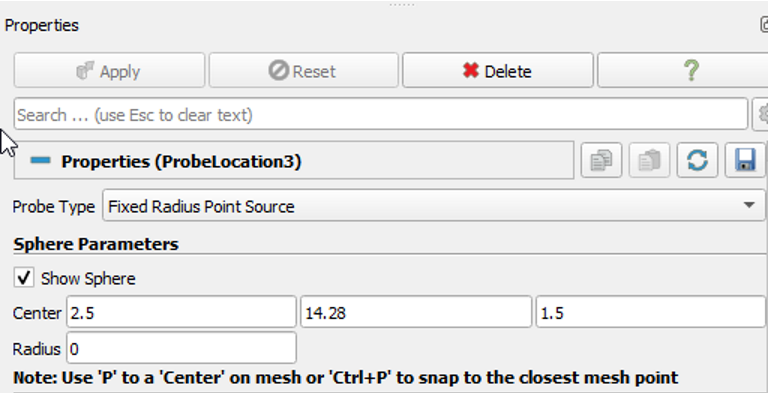
Make sure that the Radius is set to zero. Then click apply.
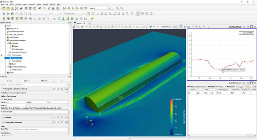
In the above image we have added a ruler so you can get a better idea of where the point is. We have also opened a spreadsheetview so we can see the data at the point location. We also have our line graph from before, as well as a contour plot. You can see that the point’s data reads Sigma3 of 4.67MPa, which matches the low point of the line graph and the dark blue region of the contour plot.
A slice taken on the side where we performed the measurements shows some areas of relatively low strain in the vicinity of the probed area.
